Using an Extended Kalman Filter for Estimating Vehicle Dynamics and Mass
In this tutorial a slip control loop for a quarter car model is developed. Various of the vehicle states (such as longitudinal speed, wheel slip, road surface friction coefficient, and mass) are not directly measurable and hence must be estimated. An extended Kalman filter is implemented to perform the estimation based on a noisy measurement of wheel angular velocity.
This tutorial assumes that the reader is familiar with the basics of the quarter car model and the extended Kalman Filter. For a discussion of the dynamic equations of a quarter car model and implementing a slip controller assuming perfect state measurement see the Slip Control of a Quarter Car Model tutorial. For a discussion of the mathematical background of the extended Kalman filter see the An Introduction to the Extended Kalman Filter tutorial. Tutorials on general Simulink usage, Kalman filters, and their implementation in Simulink, can be found on the Software Tutorials page.
The tutorial is split into the following sections,
- A Simulink Implementation.
- Discretizing the Quarter Car Model.
- Defining the EKF Equations.
- Implementing the EKF.
- Simulating The Model.
A Simulink Implementation
A Simulink model that implements a slip control loop using the extended Kalman filter developed in this tutorial is shown in Figure 1.
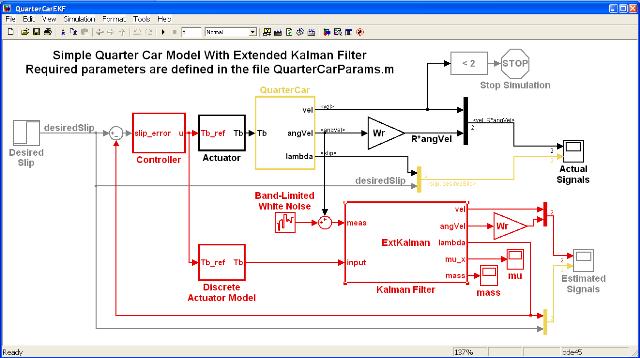
The Simulink model of Figure 1 contains a continuous time quarter car model that is used to represent the real physical vehicle and a discrete slip control loop. The slip control loop is comprised of the extended Kalman filter (developed in this tutorial) and a discrete PI controller (developed in the Slip Control of a Quarter Car Model tutorial).
A zip file containing the model of Figure 1 may be downloaded here.
Discretizing the Quarter Car Model
The standard quarter car model (as described in The Quarter Car Model) is a set of continuous time differential equations. However, the extended Kalman filter requires a set of discrete equations. Hence for use within an extended Kalman filter the quarter car model equations must be discretized.
The simplest approach for discretization is to use a forward Euler method. This lead to the discrete model
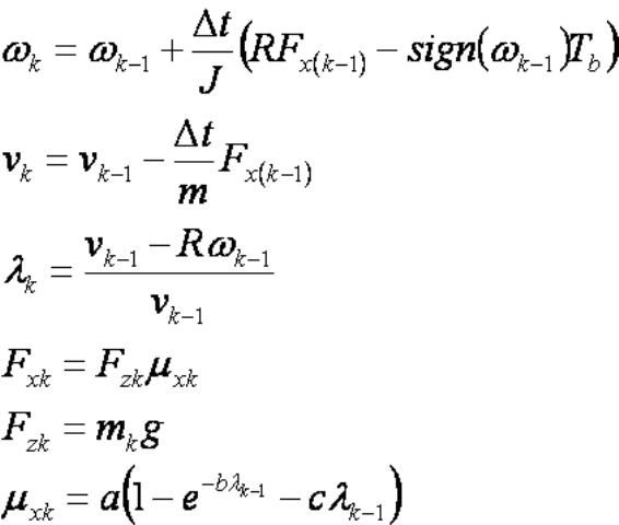
where the subscript k indicates a particular discrete point in time and k-1 indicates the previous time point. Note that Equation 1 includes not only the vehicle dynamics but also the discretized tire model.
Defining the EKF Equations
The notation used in this section follows that used to describe the mathematics behind the extended Kalman filter in the Extended Kalman Filter tutorial. Of particular importance is the requirement to define the signals that can be measured (and hence act as inputs to the extended Kalman filter) and those states that need to be estimated (by the extended Kalman filter).
In automotive applications the wheel rotational speed ω can usually be measured (albeit corrupted by noise) and for this example it is assumed to be the only measurable entity. There are however five states that it has been determined need to be estimated:
- ω – the vehicle rotational speed (filtered from the noisy measurement).
- v – the vehicle longitudinal speed.
- λ – the tire slip.
- μx – the road friction coefficient.
- m – the (quarter) vehicle mass.
The measured input and state vector to be estimated are shown in Equation 2,
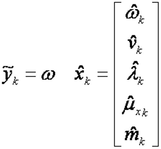
Note that some of the states in Equation 2 have been chosen arbitrarily. The vehicle longitudinal speed is a typical state that requires estimating. However including the slip, friction coefficient and particularly the vehicle mass in the states to be estimated is purely a design decision. At first glance mass in particular may be considered an unusual parameter to estimate. However, if the vehicle in question is highly configurable (i.e. is capable of carry loads that range from very heavy to very light or non-existent) then a mass estimate may be important.
The extended Kalman filter uses a two step predictor–corrector algorithm. As part of the algorithm two Jacobians are required, Fk and Hk. For the discrete quarter car model of Equation 1 with the measured input and states of Equation 2 these are,
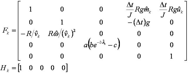
The last row of Fk indicates that the mass of the vehicle is assumed to be constant. However, due to the stochastic nature of the extended Kalman filter, it really means that the mass is allowed to be slowly varying.
Implementing the EKF
The extended Kalman filter has been implemented using an Embedded MATLAB Function block. The block is discrete with a sample time of 5ms. The code for the block is shown below.
Note that the noise covariance matrices R and Q are based upon best guestimates. In practise their values would need to be tuned based on measured data.
function [vel,angVel,lambda,mu_x,mass] = ...
    ExtKalman(meas,input,Ts,v0,m0,Wr,g,J,roadCoeffs)
%#eml
% This Embedded MATLAB Function implements an extended Kalman filter used
% to estimate the states, road surface and mass of a quarter car model.
%
% The states of the process are given by
% x = [omega;velocity;slip;road friction;mass];
%
% There is assumed to be one measurement
% y = [omega]
%

% Author: Phil Goddard (phil@goddardconsulting.ca)

% Define storage for the variables that need to persist
% between time periods.
persistent P xhat Q R
if isempty(P)
   % First time through the code so do some initialization
   xhat = [v0/Wr;v0;0;0;m0];
   P = zeros(5,5);
   Q = diag([0.01^2 0.01^2 1 1 0.001^2]);
   R = 0.005/Ts;
end
% Calculate the Jacobians for the state and measurement equations
F = [1 0 0 Ts*(1/J)*(Wr*g*xhat(5)) Ts*(1/J)*(Wr*g*xhat(4));
     0 1 0 Ts*(-g) 0;
     -(Wr/xhat(2)) Wr*xhat(1)/(xhat(2)^2) 0 0 0;
     0 0 roadCoeffs(1)*...
     (roadCoeffs(2)*exp(-roadCoeffs(2)*xhat(3))-roadCoeffs(3)) 0 0;
     0 0 0 0 1];
H = [1 0 0 0 0];
% Propogate the state and covariance matrices
xhat = [...
    xhat(1) + Ts*(1/J)*(Wr*g*xhat(4)*xhat(5) - sign(xhat(1))*input);
    xhat(2) + Ts*(-g*xhat(4));
    (xhat(2) - Wr*xhat(1))/xhat(2);
    roadCoeffs(1)*(1 - exp(-roadCoeffs(2)*xhat(3))-roadCoeffs(3)*xhat(3));
    xhat(5)];
P = F*P*F' + Q;
% Calculate the Kalman gain
K = P*H'/(H*P*H' + R);
% Calculate the measurement residual
yhat = xhat(1);
resid = meas - yhat;
% Update the state and covariance estimates
xhat = xhat + K*resid;
P = (eye(size(K,1))-K*H)*P;
% Post the results
vel = xhat(2);
angVel = xhat(1);
lambda = xhat(3);
mu_x = xhat(4);
mass = xhat(5);
Simulating The Model
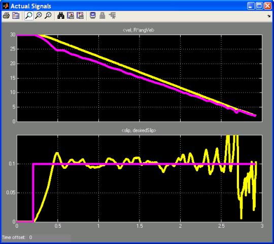
The results of simulating the model of Figure 1 with the extended Kalman filter of Figure 2 are shown below. Figure 3 shows the signals output by the real continuous time vehicle, while Figure 4 shows the signals estimated by the extended Kalman filter. It is these estimated signals that are fed back to the controller to form the slip control loop.
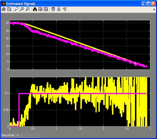
Note that the estimated slip is quite noisy. This isn’t untypical of real slip data, however in the simulation it could possibly be reduced by better tuning of the noise covariance matrices R and Q.
|
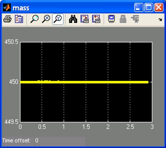
A final comment should be made regarding the vehicle mass estimate. Figure 5 shows a plot of the estimated mass. It is initialized to 450Kg which is the same as the actual vehicle mass and it does not substantially change. Over the 3s of this simulation the mass shouldn’t be expected to change. Only over a longer time frame, where the model is designed to take account of fuel use or variable loads, would a change be expected to be noticed. |
This tutorial has discussed the implementation in Simulink of an extended Kalman filter for estimating various states of an automotive quarter car model and using them as part of a slip control loop. Other Simulink tutorials are available on the Software Tutorials page.