An Introduction to the Extended Kalman Filter

Kalman Filters are a form of predictor-corrector algorithm used extensively in control systems engineering for estimating unmeasured states of a process. The estimated states may then be used as part of a strategy for control law design.

This tutorial discusses the Extended Kalman Filter which was developed for non-linear discrete-time processes (or at least processes that may be modeled with sufficient accuracy as a non-linear discrete-time process). Other tutorials discuss other types of Kalman filters: the original Kalman Filter (for linear processes); the Kalman-Bucy Filter (for continuous-time systems); and the Unscented Kalman Filter (which is an extension of the Extended Kalman Filter).

Figure 1: Non-linear discrete-time process with input and measurement noise.

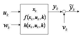
Consider the non-linear discrete-time process shown in Figure 1 which may be written in the standard state-space form,

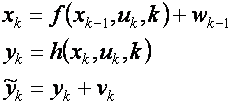
Here

• k denotes a discrete point in time (with k-1 being the immediate past time point).
• u_k is a vector of inputs
• x_k is a vector of the actual states, which may be observable but not measured.
• y_k is a vector of the actual process outputs.
• is a vector of the measured process outputs.
• w_k and v_k are process and output noise respectively. They are assumed to be zero mean Gaussian with covariance Q_k and R_k respectively.
• f(.) and h(.) are generic non-linear functions relating the past state, current input, and current time to the next state and current output respectively.

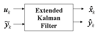
Given the inputs, measured outputs and assumptions on the process and output noise, the purpose of the Extended Kalman Filter is to estimate unmeasured states (assuming they are observable) and the actual process outputs. This is shown in Figure 2 where the estimated states are , and are the estimated measured outputs.

Figure 2: Input-output of the Extended-Kalman Filter.

As with the original Kalman Filter, the Extended Kalman Filter uses a 2 step predictor-corrector algorithm. The first step involves projecting both the most recent state estimate and an estimate of the error covariance (from the previous time period) forwards in time to compute a predicted (or a-priori) estimate of the states at the current time. The second step involves correcting the predicted state estimate calculated in the first step by incorporating the most recent process measurement to generate an updated (or a-posteriori)state estimate.

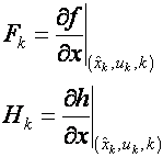
However, due to the non-linear nature of the process being estimated the covariance prediction and update equations cannot use f and h directly. Rather they use the Jacobian of f and h. The Jacobians are defined as

For the Extended-Kalman Filter, mathematically, the predictor step is given by

And the corrector step is given by,

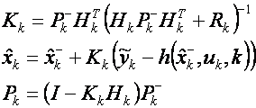
In the above equations P_k is an estimate of the covariance of the measurement error and K_k is called the Kalman gain. After both the prediction and correction steps have been performed then is the current estimate of the states and can be calculated directly from it. Both and P_k are stored and used in the predictor step of the next time period.

If the process is linear then the above equations collapse to the equations of the original (i.e. linear) Kalman Filter. However, unlike the Kalman Filter, the Extended-Kalman Filter is not optimal in any sense. And further, if the process model is inaccurate then due to the use of the Jacobians -- which essentially represent a linearization of the model -- the Extended-Kalman Filter will likely diverge leading to very poor estimates.

However, in practise, and when used carefully, the Extended-Kalman Filter can lead to very reliable state estimation. This is particularly the case when the process being estimated can be accurately linearized at each point along the trajectory of the states.

A simple example demonstrating how to implement an Extended Kalman Filter in Simulink can be found here.

Back To Top | Kalman Filters