Option Pricing - Monte-Carlo Methods
Monte-Carlo methods are ideal for pricing options where the payoff is path dependent (e.g. lookback options, asian options and spread options) or options where the payoff is dependent on a basket of underlying assets (rather than just a single asset).
This tutorial discusses the fundamental mathematical concepts behind Monte-Carlo methods. Other tutorials discuss variance reduction techniques for increasing the efficiency of Monte-Carlo simulation, pricing options that are dependent on a basket of underlying assets, and the Longstaff-Schwartz approach for using Monte-Carlo techniques to price American style options. Tutorials showing how to apply Monte-Carlo techniques for pricing several different types of options, implemented in MATLAB, may be found on the Software Tutorials page.
As with other option pricing techniques Monte-Carlo methods are used to price options using what is esentially a three step process. The three steps are,
- Calculate potential future prices of the underlying asset(s).
- Calculate the payoff of the option for each of the potential underlying price paths.
- Discount the payoffs back to today and average them to determine the expected price.
Monte-Carlo methods differentiate themselves from other option pricing techniques in the way that potential future asset prices are generated. The following Simulating Asset Paths section describes how these paths may be generated for a standard log-normal model of equity asset prices. However, the technique may be applied to any asset that follows any stochastic process (where an associated random distibution exists from which samples may be obtained).
Simulating Asset Paths
The first step in using Monte-Carlo methods is to generate (a large number of) potential future asset prices. This is done by selecting an appropriate (stochastic) model for the time evolution of the underlying asset(s) and then simulating the model through time.
For example, the standard model for evolution of equity prices is given by the Weiner process.

where,
- S(0): The stock price today.
- S(Δt): The stock price at a (small) time into the future.
- Δt: A small increment of time.
- μ: The expected return.
- σ: The expected volatility.
- ε: A (random) number sampled from a standard normal distribution.
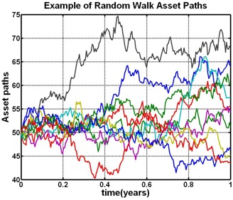
Repeated use of Equation 1 allows multiple potential future asset paths (between now and expiry) to be generated. An example of 10 such paths is given in Figure 1. The underlying price at each time step along each path is generated by repeatedly sampling from a standard normal distribution and applying Equation 1.
Typically many thousands, if not tens of thousands, of simulated paths must be generated to enable an accurate option price to be calculated. The more paths that are generated the longer the simulation will take to be performed and hence the longer the time taken to price the option. Variance reduction technqiues have been developed in an attempt to minimize the number of simulations required to generate an accurate option price.

When an option is dependent on a basket of underlying assets then multiple correlated assets paths must be simulated. How to generate appropriate correlated paths is discussed in the Correlated Simulation Paths tutorial.
Pricing the Option
Once the asset paths have been simulated they are used to price the option according to the option's payoff formulae.
For instance, consider a simple Asian option where the payoff is a function of the average price of the underlying asset over the life of the option. For put and call options the payoff is

where A is the average value of the asset price over the life of the option and X is the strike.
The price of an Asian option is calculated using Monte-Carlo simulation by performing the following 4 steps
- averaging the asset price for each of the simulated paths.
- applying the appropriate formula of Equation 2.
- averaging the payoffs for all paths.
- discounting the result back in the usual way.
An example of implementing the above procedure in MATLAB is given in the Pricing an Asian Option in MATLAB tutorial. Other MATLAB based Monte-Carlo tutorials are linked off the Software Tutorials page.