A Simple Kalman-Bucy Filter in Simulink
This tutorial presents a simple example of how to implement a Kalman-Bucy filter in Simulink. If you are unfamiliar with the mathematics behind the Kalman Filter or the Kalman-Bucy filter then see these tutorials.
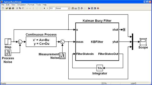
A Simulink model that implements a simple Kalman-Bucy Filter using an Embedded MATLAB Function block is shown in Figure 1. The purpose of this model is to show how a Kalman-Bucy Filter may be used to identify any unmeasured states of a continuous time process using only the process input signal and a noisy measured output..

The process under consideration is a simple first order, time-invariant system given by the following set of equations,

The above model is equivalent to the continuous time transfer function

and hence should track a step input with zero steady-state error.
The process model is subject to two sources of zero-mean Gaussian noise. The input is corrupted with noise having a variance of 0.01 and the output is corrupted with noise having a variance of 0.1.
Note that for this model the state and the output are scaled versions of each other so the terms can be used interchangeably. Hence although both the estimated state and output have been calculated by the Kalman-Bucy Filter only the estimated output is being displayed on the Scope.
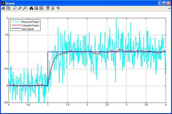
The input signal, measured output and estimated output are displayed on the Scope. This is shown in Figure 2.
Note that the Kalman-Bucy filter does a good job of rejecting the noise and estimating a signal that accurately tracks the step input.

The Kalman-Bucy Filter itself has been implemented in an Embedded MATLAB Function block. The code within that block is shown below.
function [xhat,yhat, FilterStatesOut] = KBFilter(u,meas,FilterStatesIn)
% This Embedded MATLAB Function implements a very simple Kalman Bucy filter.
%
% The filter estimates both the state and output of a linear,
% continuous-time, time-invariant, system given by the following
% state-space equations:
%
% xdot = -9*x + 3*u + w
%    y = 3*x + v
%
% where w and v are zero-mean Gaussian noise with variance of 0.01 and 0.1
% respectively.

% Author: Phil Goddard (phil@goddardconsulting.ca)
% Date: Q2, 2011.

% preallocate outputs
nstates = 1;
xhat = 0;
yhat = 0;
FilterStatesOut = zeros(2*nstates,1); %#ok
% Model parameters
A = -9;
B = 3;
C = 3;
Q =  0.01; % Process noise
R =  0.001; % Measurement noise
% Separate out the model state estimate and the
% Kalman Filter states
xhat = FilterStatesIn(1:nstates);
P = FilterStatesIn(nstates+1:end);
% calculate the residual
residual = meas - C*xhat;
% Calculate the filter gain
K =(P*C')/R;
% state update equations
xhatdot = A*xhat + B*u + K*residual;
Pdot = A*P +P*A' - K*R*K' + Q;
% assign outputs
yhat = C*xhat;
FilterStatesOut = [xhatdot;Pdot];
The main purpose of this tutorial is to demonstrate a Simulink implementation of the Kalman-Bucy Filter equations. The process model under consideration has deliberately been chosen to be very simple, and consequently the Kalman-Bucy filter does a good job at rejecting the process and measurement noise to generate a very good estimate of the process output.
Other tutorials discuss the Kalman Filter and its application for state estimation and in estimating unknown model parameters for discrete-time processes.