Option Pricing - Alternative Binomial Models
This tutorial discusses several different versions of the binomial model as it may be used for option pricing. A discussion of the mathematical fundamentals behind the binomial model can be found in the Binomal Model tutorial. As introduced in that tutorial there are primarily three parameters -- p, u and d -- that need to be calculated to use the binomial model.
The Binomal Model tutorial discusses the way that p, u and d are chosen in the formulation originally proposed by Cox, Ross, and Rubinstein. In the tutorials presented here several alternative methods for choosing p, u and d are presented. The methods discussed here are those proposed by,
- Jarrow-Rudd: This is commonly called the equal-probability model.
- Tian: This is commonly called the moment matching model.
- Jarrow-Rudd Risk Neutral: This is a modification of the original Jarrow-Rudd model that incorporates a risk-neutral probablity rather than an equal probability.
- Cox-Ross-Rubinstein With Drift: This is a modification of the original Cox-Ross-Runinstein model that incorporates a drift term that effects the symmetry of the resultant price lattice.
- Leisen-Reimer: This uses a completely different approach to all the other methods, relying on approximating the normal distrbution used in the Black-Scholes model.
Jarrow-Rudd
For reasons that will become self-evident, the binomial model proposed by Jarrow and Rudd is often refered to as the equal-probability model.
In the Binomal Model tutorial two equations are given that ensure that over a small period of time the expected mean and variance of the binomial model will match those expected in a risk neutral world. Since there are three unknowns in the binomial model (p, u and d) a third equation is required to calculate unique values for them.
The third equation proposed by Jarrow and Rudd is
![]()
and hence there is an equal probability of the asset price rising or falling.
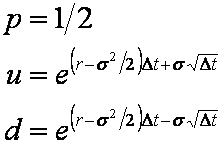
This leads to the equations,

The p, u and d calculated from Equation 2 may then be used in a similar fashion to those discussed in the Binomal Model tutorial to generate a price tree and use it for pricing options. Note that a consequence of Equation 1 is that the Jarrow-Rudd model is no longer risk neutral. The alternative Jarrow-Rudd Risk Neutral model, discussed shortly, addresses this drawback.
Tian
In the Binomal Model tutorial two equations are given that ensure that over a small period of time the expected mean and variance of the binomial model will match those expected in a risk neutral world. Note that the mean an variance are called the first and second moments of a distribution.
The model proposed by Tian exactly matches the first three moments of the binomial model to the first three moments
of a lognormal distribution.
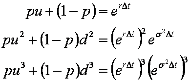
Hence the three equations used by Tian are

This leads to the parameters,

The p, u and d calculated from Equation 4 may then be used in a similar fashion to those discussed in the Binomal Model tutorial.
Jarrow-Rudd Risk Neutral
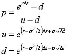
The Jarrow-Rudd Risk Neutral model is a minor modification to the standard Jarrow-Rudd model. The same u and d are used, however instead of p=1/2 the standard risk neutral value for p is chosen.
This gives the following parameters,

The p, u and d calculated from Equation 4 may then be used in a similar fashion to those discussed in the Binomal Model tutorial. This model is a special case of the Cox-Ross-Rubinstein With Drift model.
Cox-Ross-Rubinstein With Drift
The derivation of the original binomial model equations as discussed in the
Binomal Model tutorial holds even when an arbitrary drift is
applied to the u and d terms.
Hence, for an arbirary η, the following parameters give a valid binomial model

When the drift term η is set to the zero this model collapses to the original Cox-Ross-Rubinstein binomial model which generates a lattice of prices that is centred around the current asset price S0. This is shown in Figure 3 of the Binomal Model tutorial.
However, with the original model, if the option is a long way out of the money then only a few of the resulting lattice points may have a non-zero payoff associated with them at expiry. The drift term can be used to drift (or skew) the lattice upwards or downwards to obtain a lattice where more of the nodes at expiry are in the money.
The Jarrow-Rudd Risk Neutral model is a specific case of the Cox-Ross-Rubinstein With Drift model. A common drift is η = (ln(X)-ln(S0))/T, (where ln(·) is the natural logarithm and T is the time to expiry in years) which makes the resulting lattice symmetric about the strike at expiry. A drawback of that particular drift is that the underlying price tree is a function of the strike and hence must be recalculated for options with different strikes, even if all other factors remain constant.
Leisen-Reimer
Leisen and Reimer developed a model with the purpose of improving the rate of converegence of their binomial tree. (All of the models discussed above converge to the Black-Scholes solution in the limit as the size of the time step Δt is reduced to zero. However the convergence is not smooth.)
The Leisen-Reimer tree is generated using the parameters,

where h-1(·) is a discrete approximation to the cummulative distribution function for a normal distribution. There are several ways this can be calculated. One suggested by Leisen and Reimer is to use,

where n is the number of time points in the model (including times 0 and T) which must be odd, and d1 and d2 are their usual definitions from the Black-Scholes formulation.